


You know how it is - in OMSI there are many maps, whether real or fictitious, but you are always missing that one special map - the local bus line. In this guide I describe step by step how to put an end to this annoying issue. Please note that for this tutorial you need to have a certain basic knowledge of 3D modelling. In this tutorial we will deal with the import of aerial photographs.
1. Preparation
To start with the development we need the following programmes:
- Blender 2.7x (Download: https://download.blender.org/release/) (in the tutorial I only work with Blender 2.79)
- SAS.Planet (Download: http://www.sasgis.org/)
Next we need a project folder. In this folder the needed aerial photos will be saved later, Blender accesses this folder permanently, but pay attention to the place where you want to save it.
As a last step of preparation you should already have an exact idea of which section or route you want to save. A correction is no longer possible. You should also have a stable connection to download high-resolution images.
It is also recommended to create a folder in "OMSI2\Sceneryobjects" in which textures are already prepared for the later road and intersection objects.
1.1. Checklist
- Internet line is stable enough
- Blender downloaded
- Downloaded SAS.Planet
- Created a project folder that is safe and that Blender can access permanently.
- (Recommendation: create OMSI Sceneryobjects folder)
- Track layout is clear
2. SAS.Planet
2.1. Launch SAS.Planet
We start SAS.Planet. To do this, open the EXE "SASPlanet.exe" by double-clicking on it (Fig. 1). A dialogue screen appears, then the user interface opens (Fig. 2).

Fig. 1
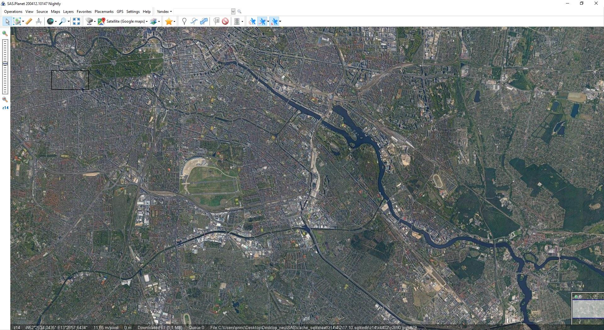
Fig. 2
Navigate to the starting point
In SAS.Planet we now navigate to our starting point. Using the dropdown menu, which opens when you click on "Yandex" as the first selection, you can select various sources to navigate to the starting point. I use the menu item "URL". In the adjacent field, links can be entered that carry a reference value. (Fig. 5)
In addition, if not set, "Satellite (Google maps)" must be selected as the source (Fig. 6).
In my case I enter the following link: (Fig. 4)
This link contains all the important information so that SAS Planet can find my place of reference where I want to start my work.
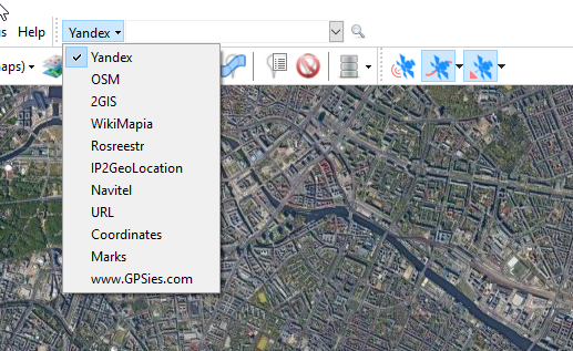
Fig. 3
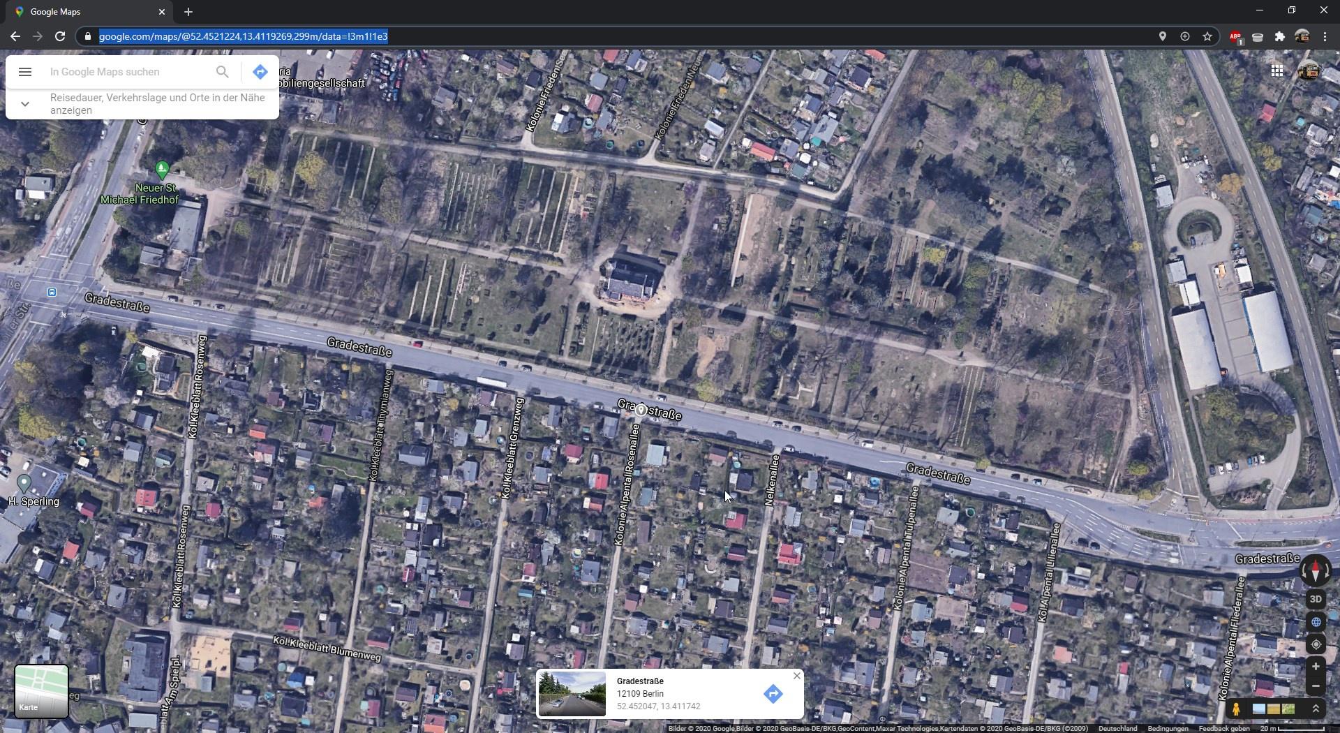
Fig. 4
Fig. 5
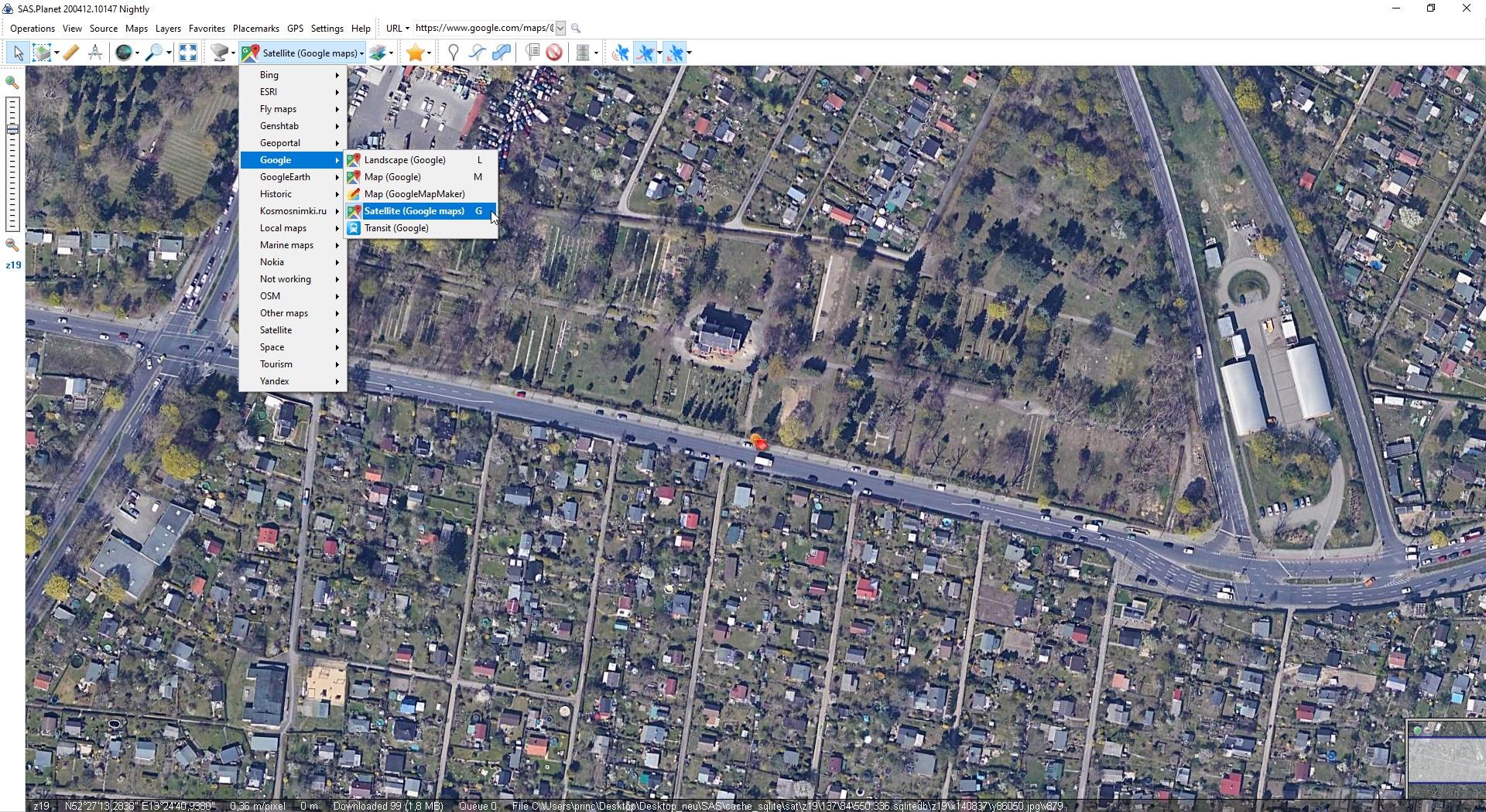 Fig. 6
2.2. Selection
Next, we mark the area that we would like to download afterwards. We can use different methods to mark our area.
You can choose from the following: (Fig. 7)
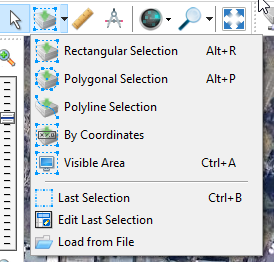
Fig. 7
In my case I use the polygonal selection. With this method I can set more than 4 points to mark my area. At the end, every "tile" that is in the marked area is downloaded.
Via a small menu that pops up when you set the first point, four more options can be used. The option on the left deletes the last point "touched" with the mouse - not the last point set. (Fig. 8)
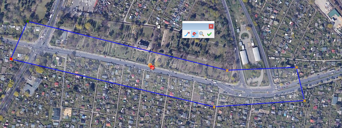
Fig. 8
2.3. Downloading the data
After we have selected our area, we confirm it by clicking on the green arrow - far right (Fig. 8). A new window appears - the "Selection Manager". Here we set our source (which is already set by our selection of the layer) and our zoom height. This is important for our resolution later on the aerial photos. I use the option "21" for this (Fig. 9).
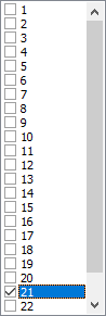
Fig. 9
Next, the "Start" button must be pressed, SAS-Planet starts downloading the individual "tiles". (Fig. 10)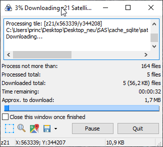
Fig. 10
Attention! It can happen that the download stops at some point if you obtain too much data from the Google server in a short time. In this case, Google no longer likes your IP address. As a solution, you can use a VPN (I use NordVPN for this) to simply connect to a new server and continue.
2.4. Save
As soon as the download is complete, you must click on the blue-dashed box at the bottom left (Fig. 11).
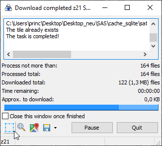
Fig. 11
The Selection Manager opens again, but this time we change the tab to "Stitch". Once there, we assign a storage location by clicking on the three boxes in the grey area. Then we click on Start and SAS.Planet saves an image file to the specified location. (Fig. 12)
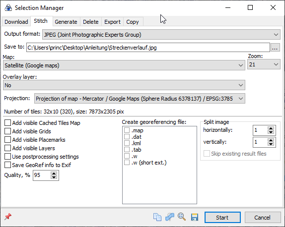
Fig. 12
Caution: If the image becomes too large (limit values are under the item: "Projection"), the "large" image must be split. For this purpose, values above 1 must be entered for the respective axis under "Split image". (Fig. 13)
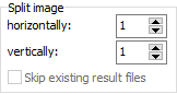
Fig. 13
After we have saved the image, the Selection Manager disappears. Before we close SAS.Planet we need the zoom factor. This can be found at the bottom left of the image. (Fig.14)
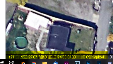
Fig. 14
For larger pictures, it is also advisable to measure the distance at two reference points using the ruler. This can be found in the upper selection bar next to the mouse cursor.
3. Blender
Now we need Blender. We open it and import our image(s). For the import, Blender has a practical plugin (Import Images as Planes), which still has to be activated. (Fig. 15)
Fig. 15
3.1. Importing the image
Now that the plugin has been activated, we import the image. The importer can be found via File -> Import -> Images as Planes (Fig. 16) alternatively via Shift+A -> Mesh -> Images as Planes (Fig. 17).
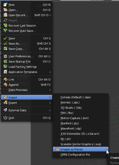
Fig. 16
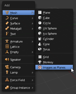
Fig. 17
3.2. Fitting the size
Once the image(s) is/are imported, we switch to Material Mode in Blender and activate the Environment Lighting option (Fig. 18).

Fig. 18
Now we need our zoom factor. In my case it is 0.09 m/pixel. To be able to use this value, we need the width and height of our image(s) (it is always the same). To do this, right-click on the file -> Properties and switch to the tab "Details". Under the title "Image" we find our necessary dimensions (Fig. 19).
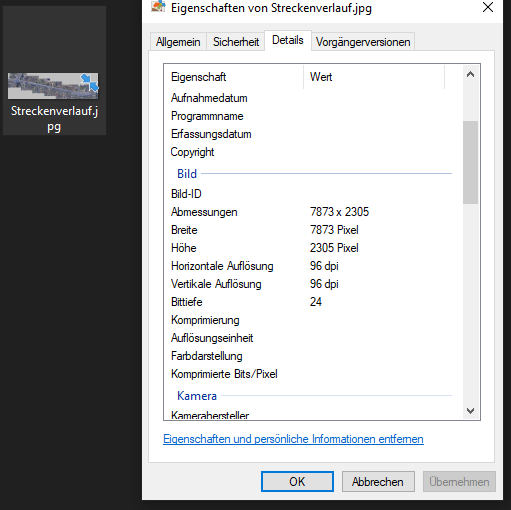
Fig. 19
Back in Blender we now use our values to bring the image to the correct dimensions. The following steps are taken: Take one of the values, I use 7873 Px as the width and multiply this by 0.09. This is entered in Blender in the field "Dimensions". This can be called up via the N key and is displayed when the object is selected. (Fig. 20)
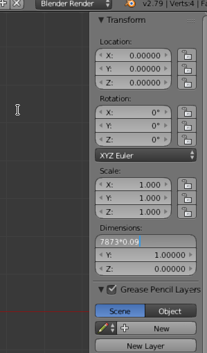
Fig. 20
Blender now spits out a result. The generated value at "Scale", one table above, is our new scale value. This must now be copied and entered at Y (or X, as the case may be). As a check, the second value can be calculated and compared with the zoom factor in Y. It should be identical, otherwise it is not. It should be identical, otherwise the first calculation is not correct. (Fig. 21)
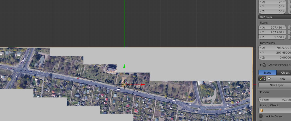
Fig. 21
4. Completion
The object is now imported into Blender and we can start creating our roads and intersections. If several images are needed, they can be imported and enlarged again and again with the same scale value. In order to line up the images correctly, we recommend setting the snap element to vertex (fig. 22). This way, arranging the images should not be a problem.
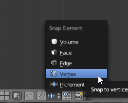
Fig. 22
Thank you for reading through, I hope the approach to creating your own maps is a motivational boost. A tutorial on how to create street and intersection objects as I build them will be added if necessary.
")